Reliability & Maintenance Analyst - Data Entry Grid
|
Reliability & Maintenance Analyst - Data Entry Grid |
|
The File option of the main menu provides functions related to getting data in and out of the software. All options are standard with the exception of the New option and the Reporting option. New Select this option to enter data using the data entry screen. The
user is prompted for the type of data to be entered -
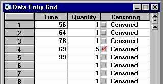
individual or grouped. The "New" icon When a cell is in edit mode the menu is disabled. Press the enter key, or click another cell to enable the menu. Individual Data The Individual Data entry grid, shown in the figure below, is used when the time to fail or the censoring time is known for all items in the data set. If the number of failures in a given time interval is known, but exact failure times are not known, use the Grouped Data entry grid. The default number of rows in the grid is 5000, but up to 2 billion rows can be added using the "Specify Number of Rows" entry on the "Edit" menu. There are three columns in the Individual Data entry grid:
There are three limits when using individual data:
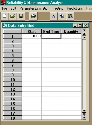
When using the individual data grid there should not be more than 1 data point with the same failure time. This occurs when testing is monitored on an interval basis rather than continuously. It is best to use the grouped data procedures for this type of data collection. It is recommended to use the grouped data format if there are more than 1 million data points. Although the individual data grid allows 2 billion data points, execution time becomes large if the number of data points is greater than 1 million. The Grouped Data entry grid, shown in the figure below, is used if exact failure times are not known, but the number of failures in an interval is known. There are 3 columns in the Grouped Data entry grid:
The starting time of the first interval is assumed to be zero, and the starting time of each successive interval is set equal to the ending time of the previous interval. The value of the quantity must be greater than zero. The cumulative distribution function is not estimated from the last interval, it is only used to determine the total number of units tested. For example, consider the data shown in the figure below.
In this example, the test began with 30 items (3+5+1+21). After testing for 10 time units, 3 items had failed. After testing 20 time units, 5 additional units failed, for a total of 8 failures. After testing 30 time units, 1 additional unit failed, for a total of 9 failures, and testing was ceased. Since 30 units were tested, the additional 21 units are placed in the last cell. The "End Time" of 40 is arbitrary and has no meaning. The only restriction is that it is greater than the "Start Time" in the same row. When using grouped data the only method of parameter estimation available is probability plotting. Also, there are no confidence limits on the probability plot. When grouped data is used, the sample sizes are typically so large that any confidence interval computed is very small. |