|
|
Below is a step by step example of how to determine reliability confidence
limits. The example utilizes the Reliability & Maintenance
Analyst software. Click here to download a free demo version of
this software.
Click here for the technical details of
the determining reliability confidence limits using the Weibull
distribution in Adobe Acrobat format. For the same
article in Microsoft Word for Windows 95 format click
here.
Ten units are placed on a test stand. The following failures were
recorded
| Cycles to Fail |
| 283,121 |
| 317,982 |
| 264,764 |
| 451,384 |
| 501,236 |
Of the remaining 5 units, two were removed from testing without failing after 300,000
cycles, and three were removed from testing after 600,000 cycles without failing.
A. Compute the lower 80% confidence limit for reliability at 200,000 cycles.
B. Compute the lower 80% confidence limit for the time to fail at 99% reliability.
Solution
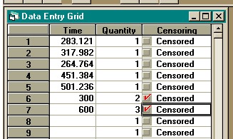
- Enter the data into the "Individual Data" entry grid. When doing this,
calculations are executed faster when smaller number are used. In this example, it
is best to enter the data as "thousands". For example instead of entering
283,121 cycles, enter 283.121 cycles, and instead of entering 300,000 cycles, enter 300
cycles. The items that did not fail must be entered as censored. This is done
by checking the "censored" box. Note that a quantity of 2 is entered in
row 6 indicating that 2 units survived for 300 thousand cycles without failing. A
quantity of 3 is entered in row 7 to indicate that 3 units survived for 600 thousand
cycles without failing. This is shown in the figure below.
- The correct distribution to model the data must be determined. This is done with a
visual goodness-of-fit test using either a probability plot or a hazard plot. If the
plotted points follow the straight line in the plot, then the chosen distribution
adequately models the data. If not, then another distribution must be chosen.
The first distribution chosen to model time to fail data is usually the Weibull
distribution, followed by the lognormal and then the normal distributions. The
exponential distribution is a special case of the Weibull distribution, thus, if the
Weibull distribution does not adequately model the data then the exponential distribution
will also to fail to model the data. Select "Weibull" then
"Probability Plot" from the "Parameter Estimation" menu to obtain a
probability plot estimation. Then click the "Plot" button to obtain the
plot. This is shown in the figure below.
If you are unsure if the points follow the straight line well enough for the chosen
distribution to provide an adequate estimation model, use the random number generation
tool that can be found under the "File" menu. Simply generate a number of
random data points equal to the number of failures (5 in this case) from the same
distribution with the same parameters as shown on your probability plot screen, and generate a probability plot with the simulated data. Since the data is
simulated, you know the distribution models the data perfectly, and you can compare the
probability plot obtained using simulated data to the probability plot of your data. Try using 4 or 5 simulated
data sets for comparison. This will provide a good feel for how the probability plot
looks when the distribution adequately models the data.
- The points on the probability plot follow the straight line, so the Weibull distribution
is accepted as a model. Maximum likelihood is known to be more accurate than
probability plotting, so maximum likelihood will be used for all estimates. The only
purpose of the probability plot was to determine goodness-of-fit. Before continuing,
copy the probability plot to the clipboard using the copy icon. The plot will be
included in a report later in the example. To estimate the parameters of the Weibull
distribution using maximum likelihood estimation select "Weibull" and
"Maximum Likelihood (MLE)" from the "Parameter Estimation" menu.
The following screen will be generated.
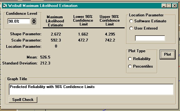
Notice that the estimated parameters are different than the estimations obtained from
probability plotting. The MLE estimates are more accurate.
- Select "Weibull" from the "Predictions" menu. Change the
confidence level from 90% to 80% in the "Confidence Level" frame at the upper
left hand of the screen. You must press the "Enter" key after changing the
confidence level for it to take effect. A message box will be displayed when you
depress the "Enter" key. The confidence level being used is shown in the
title bar of the spreadsheet at the bottom of the screen. Click the spreadsheet in
the first row under the "Time" column and enter 200. After entering 200
press the down cursor or press the "Enter" key. The lower confidence limit
for reliability at time = 200 thousand cycles is given to be 0.8773. This means that
you are 80% sure that at least 87.73% of the population will survive for at least 200,000
cycles. Click the second row of the spreadsheet under the "Reliability"
column, and enter 0.99. The lower 80% confidence limit for the time to fail at 99%
reliability is 63,560 cycles. This means that you are 80% sure that 99% of the
population will survive for at least 63,560 cycles.
- Click the icon that looks like a printer. This will open a report with the current
data. Click the paste icon, and the probability plot will be placed in the report.
This is a fully-functional wordprocessor. Saving the file in rich text format
will allow this file to be opened by any other Windows based wordprocessor. This is
shown below.
|
