Weibull Bayesian Estimation

	Weibull Bayesian Estimation

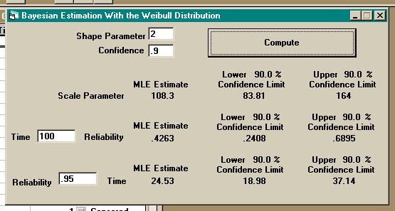
Bayesian estimation is tedious and computer routines are often employed. Commercial software is available for these calculations, such as the Reliability & Maintenance Analyst.

The following section describes bayesian estimation using the Reliability & Maintenance Analyst. The manual method is located here.

If the shape parameter of the Weibull distribution is known, it is possible to estimate the scale parameter based on this knowledge. The known shape parameter is used to transform the failure data into an exponential form. The figure below shows the bayesian estimation screen for the Weibull distribution. This screen was produced using a shape parameter of 2 and the data in the file "Demo2.dat".

bayesian.jpg (47990 bytes)

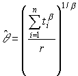
As seen from the figure above, the scale parameter is estimated with upper and lower confidence limits. If a time is entered, reliability is estimated with upper and lower confidence limits. If reliability is entered, the time is estimated with upper and lower confidence limits. Unlike other routines, this routine does not require failure data. If all the data is censored, the routine will return lower confidence limits, but not expected values or upper confidence limits.

Manual Bayesian Estimation

When using Bayesian analysis with the Weibull distribution, a data transformation can be made, and the result is data that behaves exponentially. The transformation is

Assuming the value of the shape parameter is equal to b , the maximum likelihood estimate of the scale parameter is

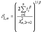
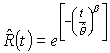
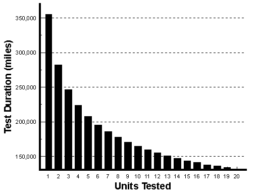
where: t_i is the time to fail or the time of censoring for the ith unit,
n is the number of units tested, and
r is the number of failures.

The lower confidence limit for the estimated scale parameter is

where: a is the level of significance (a = 0.1 for 90% confidence), and

is the critical value of the chi-square distribution with significance a , and n degrees of freedom

This expression assumes testing is discontinued after a predetermined amount of time. If testing is discontinued after a predetermined number failures, the degrees of freedom for the chi-square statistic is 2r.

The estimated reliability at time t is

The lower confidence limit for reliability at time t is

Using the above expressions, it can be seen that the test time required to demonstrate a specified reliability, at time t, with confidence 1–a , and assuming no units fail, is

where q is the characteristic life corresponding to the required reliability at time = t, and is

The duration of the test time is not directly inversely proportional to the number of units tested. The figure below shows the relationship between test duration and sample size for a verification test requiring 95% reliability with 90% confidence at 100,000 miles, assuming a shape parameter of 3.

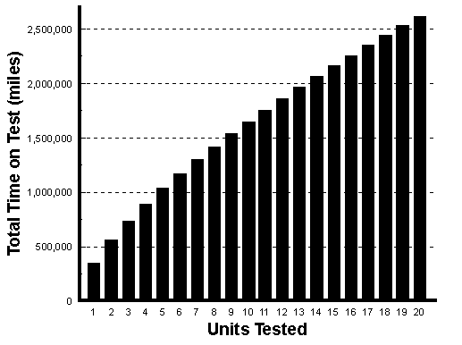
Test duration versus number of units tested to ensure 95% reliability with 90% confidence at 100,000 miles, given a shape parameter of 3, and no failures.

From the figure above, it can be seen that the total time on test (test duration X number of units tested), is increasing with the number of units tested. This is shown in the figure below.

Total time on test versus number of units tested to ensure 95% reliability with 90% confidence at 100,000 miles, given a shape parameter of 3, and no failures.

The behavior displayed in the figures above is unique to the case of a shape parameter greater than 1.0. If the shape parameter is equal to 1, the total time on test required to achieve a specified reliability with a given confidence is independent of the number of units tested. If the shape parameter is less than 1, the total time on test required to achieve a specified reliability with a given confidence decreases as the of the number of units tested increases.