EVOPtimizer Example

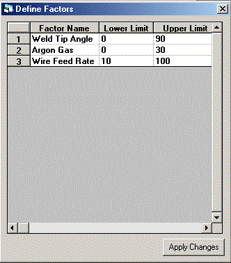
A welding process has been producing 2.3% scrap for many months.  The key factors of the process, their current settings and theoretical limits are shown below.

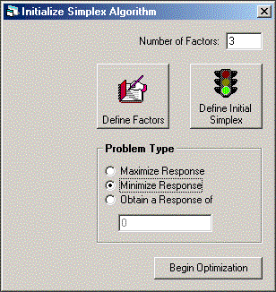
1. Set the number of factors to 3, and select Minimize Response as the problem type.  This is shown in the figure below.
   
   
   

2. Click the Define Factors button and define the factors as shown in the figure below.
   
   
   

3. Click the Apply Changes button, and the screen shown in Step 1 will be shown.

4. Click the Define Initial Simplex button, and complete the form as shown below.
   
   
   
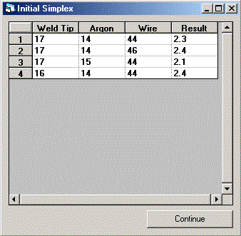
   Since there are 3 factors, the initial simplex contains 4 experiments.  We have chosen the current production setting which yielded 2.3% scrap and 3 other experiments with slight changes in 1 factor each.  The results for these additional 3 experiments are the average from several thousand trials.  It is common to run production for more than a week with an experimental setup.  If this was an experiment conducted during the research phase, the changes in the factor settings would be much wider.  They are held tight to prevent excess scrap from being produced, but the trade-off of using such small changes is that it will take longer to find the optimum settings.
   

5. Click the Continue button, and the screen shown in Step 1 will be shown.

6. Click the Begin Optimization button and the screen below will be shown.
   
   
   
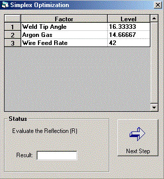
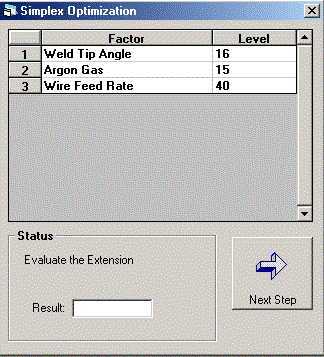
   This screen shows the next experiment.  Conduct enough trials with these factor setting to be sure the result is either better or worse than previous performance.  Enter 2.0 and click the Next Step button.
   

7. The factors settings for the next experiment are shown below.
   
   
   

8. Continue conducting experiments until you are satisfied that no further improvements can be made.

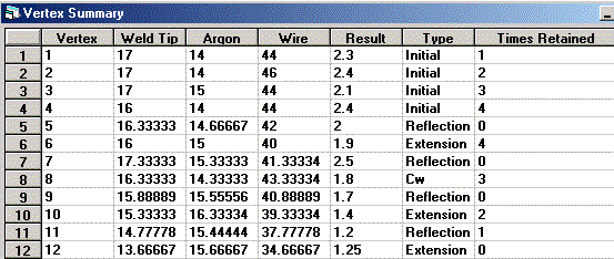
9. By selecting Vertex Summary from the Simplex menu a summary of the experimental progress can be viewed.  This is shown in the figure below.
   
   
   

10. Selecting Response Graph from the Simplex menu gives a graphical summary of the experimental progress.  This is shown in the figure below.
    
    
    
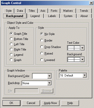
    Right-clicking anywhere on the graph dialog provides a pop-up menu to customize the graph.  This is shown in the figure below.
    
    
    
    

11. Since it may take weeks to complete the trials for each experimental setting, the problem should be saved after each step.  When a file is opened the problem will be resumed from the previous point.